![]()
Adjusting the Weights
Every node within the BMU's neighbourhood (including the BMU) has its weight vector adjusted according to the following equation:
![]()
Equation 3
Where t represents the time-step and L is a small variable called the learning rate, which decreases with time. Basically, what this equation is saying, is that the new adjusted weight for the node is equal to the old weight (W), plus a fraction of the difference (L) between the old weight and the input vector (V). My, that was a bit of a mouthful, no wonder mathematicians prefer symbols!
The decay of the learning rate is calculated each iteration using the following equation:
![]()
Equation 4
The more observant amongst you will notice that this is the same as the exponential decay function described in Equation 2, except this time I'm using it to decay the learning rate. In code it looks like this:
| m_dLearningRate = constStartLearningRate * exp(-(double)m_iIterationCount/m_iNumIterations); |
The learning rate at the start of training, constStartLearningRate, is set in the 'constants.h' file as 0.1. It then gradually decays over time so that during the last few iterations it is close to zero.
But Wait! I've not been completely honest with you. Equation 3 is incorrect! You see, not only does the learning rate have to decay over time, but also, the effect of learning should be proportional to the distance a node is from the BMU. Indeed, at the edges of the BMUs neighbourhood, the learning process should have barely any effect at all! Ideally, the amount of learning should fade over distance similar to the Gaussian decay shown below.
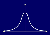
To achieve this, all it takes is a slight adjustment to Equation 3.
![]()
Equation 5
I've used the Greek capital letter theta, Θ, to represent the amount of influence a node's distance from the BMU has on its learning. Θ(t) is given by Equation 6.

Equation 6
Where dist is the distance a node is from the BMU and σ, is the width of the neighbourhood function as calculated by Equation 2. Additionally, please note that Θ also decays over time.
Some Code To Peruse
One iteration through the entire learning process is described by the Epoch method of the Csom class. This method takes a reference to the entire set of training data, picks out one input vector at random and then runs through a single iteration of the process I've described in the last few pages. Here is that method listed in its entirety. (Note that I've used distance squared values to avoid all those nasty square roots although there is loads more scope for speed improvements for all you tweakers out there.)
|
bool Csom::Epoch(const vector<vector<double> > &data) { //make sure the size of the input vector matches the size of each node's //weight vector if (data[0].size() != constSizeOfInputVector) return false;
//return if the training is complete if (m_bDone) return true;
//enter the training loop if (--m_iNumIterations > 0) { //chose a vector at random from the training set to be //this time-step's input vector int ThisVector = RandInt(0, data.size()-1);
//present the vector to each node and determine the BMU m_pWinningNode = FindBestMatchingNode(data[ThisVector]);
//calculate the width of the neighbourhood for this timestep m_dNeighbourhoodRadius = m_dMapRadius * exp(-(double)m_iIterationCount/m_dTimeConstant);
//Now to adjust the weight vector of the BMU and its //neighbours
//For each node calculate the m_dInfluence (Theta from equation 6 in //the tutorial. If it is greater than zero adjust the node's weights //accordingly for (int n=0; n<m_SOM.size(); ++n) { //calculate the Euclidean distance (squared) to this node from the //BMU double DistToNodeSq = (m_pWinningNode->X()-m_SOM[n].X()) * (m_pWinningNode->X()-m_SOM[n].X()) + (m_pWinningNode->Y()-m_SOM[n].Y()) * (m_pWinningNode->Y()-m_SOM[n].Y());
double WidthSq = m_dNeighbourhoodRadius * m_dNeighbourhoodRadius;
//if within the neighbourhood adjust its weights if (DistToNodeSq < (m_dNeighbourhoodRadius * m_dNeighbourhoodRadius)) { //calculate by how much its weights are adjusted m_dInfluence = exp(-(DistToNodeSq) / (2*WidthSq));
m_SOM[n].AdjustWeights(data[ThisVector], m_dLearningRate, m_dInfluence); }
}//next node
//reduce the learning rate m_dLearningRate = constStartLearningRate * exp(-(double)m_iIterationCount/m_iNumIterations);
++m_iIterationCount; }
else { m_bDone = true; }
return true; } |
And that's how the SOM algorithm does its magic!
Notes on the Accompanying Code
Although a colour is rendered by the computer using values for each component (red, green and blue) from 0 to 255, the input vectors have been adjusted so that each component has a value between 0 and 1. (This is to match the range of the values used for the node's weights).
You can chose to use the training set shown in Figure 1 or a training set made up of random colours by uncommenting the line "//#define RANDOM_TRAINING_SETS" found in 'constants.h'.
You should try experimenting with different values for the number of iterations and the initial learning rate to see how they effect the algorithm.
The code tweakers amongst you may like to experiment with different decay functions for the learning rate, neighbourhood radius and neighbourhood influence. There are large speed gains to be made there.